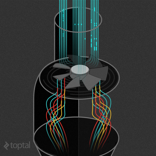
3D Data Visualization with VTK

I wrote this article on 3d data visualization with VTK for the Toptal Engineering Blog, but I’m also co-publishing it here on my own blog. The first two graphics were kindly provided by Toptal, the remaining content was created by me in close collaboration with the editor Nick McCrea.

In his recent article on Toptal’s blog, Charles Cook wrote about scientific computing with open source tools. His article makes an important point about open source tools and the role they can play in easily processing data and acquiring results.

Data visualization sketch

But as soon as we’ve solved all these complex differential equations another problems comes up. How do we understand and interpret the huge amounts of data coming out of these simulations? How do we visualize potential gigabytes of data, such as data with millions of grid points within a large simulation?

During my work on similar problems for my Master’s Thesis, I came into contact with the Visualization Toolkit, or VTK – a powerful graphics library specialized for data visualization.

In this article I will give a quick introduction to VTK and its pipeline architecture, and go on to discuss a real-life visualization example using data from a simulated fluid in an impeller pump. Finally I’ll list the strong points of the library, as well as the weak spots I encountered.

The VTK Pipeline

The open source library VTK contains a solid processing and rendering pipeline with many sophisticated visualization algorithms. It’s capabilities, however, don’t stop there, as over time image and mesh processing algorithms have been added as well. In my current project with a dental research company, I’m utilizing VTK for mesh based processing tasks within a Qt-based, CAD-like application. The VTK case studies show the wide range of suitable applications.

The VTK Visualization Pipeline

The VTK pipeline

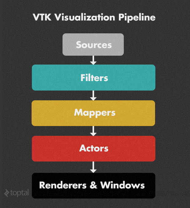
The architecture of VTK revolves around a powerful pipeline concept. The basic outline of this concept is shown here:

• Sources are at the very beginning of the pipeline and create “something out of nothing”. For example, a vtkConeSource creates a 3D cone, and a vtkSTLReader reads *.stl 3D geometry files.
• Filters transform the output of either sources or other filters to something new. For example a vtkCutter cuts the output of the previous object in the algorithms using an implicit function, e.g., a plane. All the processing algorithms that come with VTK are implemented as filters and can be freely chained together.
• Mappers transform data into graphics primitives. For example, they can be used to specify a look-up table for coloring scientific data. They are an abstract way to specify what to display.
• Actors represent an object (geometry plus display properties) within the scene. Things like color, opacity, shading, or orientation are specified here.
• Renderers & Windows finally describe the rendering onto the screen in a platform-independent way.

A typical VTK rendering pipeline starts with one or more sources, processes them using various filters into several output objects, which are then rendered separately using mappers and actors. The power behind this concept is the update mechanism. If settings of filters or sources are changed, all dependent filters, mappers, actors and render windows are automatically updated. If, on the other hand, an object further down the pipeline needs information in order to perform its tasks, it can easily obtain it.

In addition, there is no need to deal with rendering systems like OpenGL directly. VTK encapsulates all the low level task in a platform- and (partially) rendering system-independent way; the developer works on a much higher level.

Code Example with a Rotor Pump Dataset

Let’s look at an example using this dataset of fluid flow in a rotating impeller pump from the IEEE Visualization Contest 2011. The data itself is the result of a computational fluid dynamics simulation, much like the one described in Charles Cook’s article.

The zipped simulation data of the featured pump is over 30 GB in size. It contains multiple parts and multiple time steps, hence the large size. We’ll play around with the rotor part of one of these timesteps, which has a compressed size of about 150 MB.

My language of choice for using VTK is C++, but there are mappings for several other languages like Tcl/Tk, Java, and Python. If the target is just the visualization of a single data-set, one doesn’t need to write code at all and can instead utilize Paraview, a graphical front-end for most of VTK’s functionality.

The Dataset and Why 64-bit is Necessary

I extracted the rotor dataset from the 30 GB dataset provided above, by opening one timestep in Paraview and extracting the rotor part into a separate file. It is an unstructured grid file, i.e., a 3D volume consisting of points and 3D cells, like hexahedra, tetrahedra, and so on. Each of the 3D points has associated values. Sometimes the cells have associated values as well, but not in this case. We will concentrate on pressure and velocity at the points and try to visualize these in their 3D context.

The compressed file size is about 150 MB and the in-memory size is about 280 MB when loaded with VTK. However, by processing it in VTK, the dataset is cached multiple times within the VTK pipeline and we quickly reach the 2 GB memory limit for 32bit programs. There are ways to save memory when using VTK, but to keep it simple we’ll just compile and run the example in 64bit.

Acknowledgements: The dataset is made available courtesy of the Institute of Applied Mechanics, Clausthal University, Germany (Dipl. Wirtsch.-Ing. Andreas Lucius).

The Target

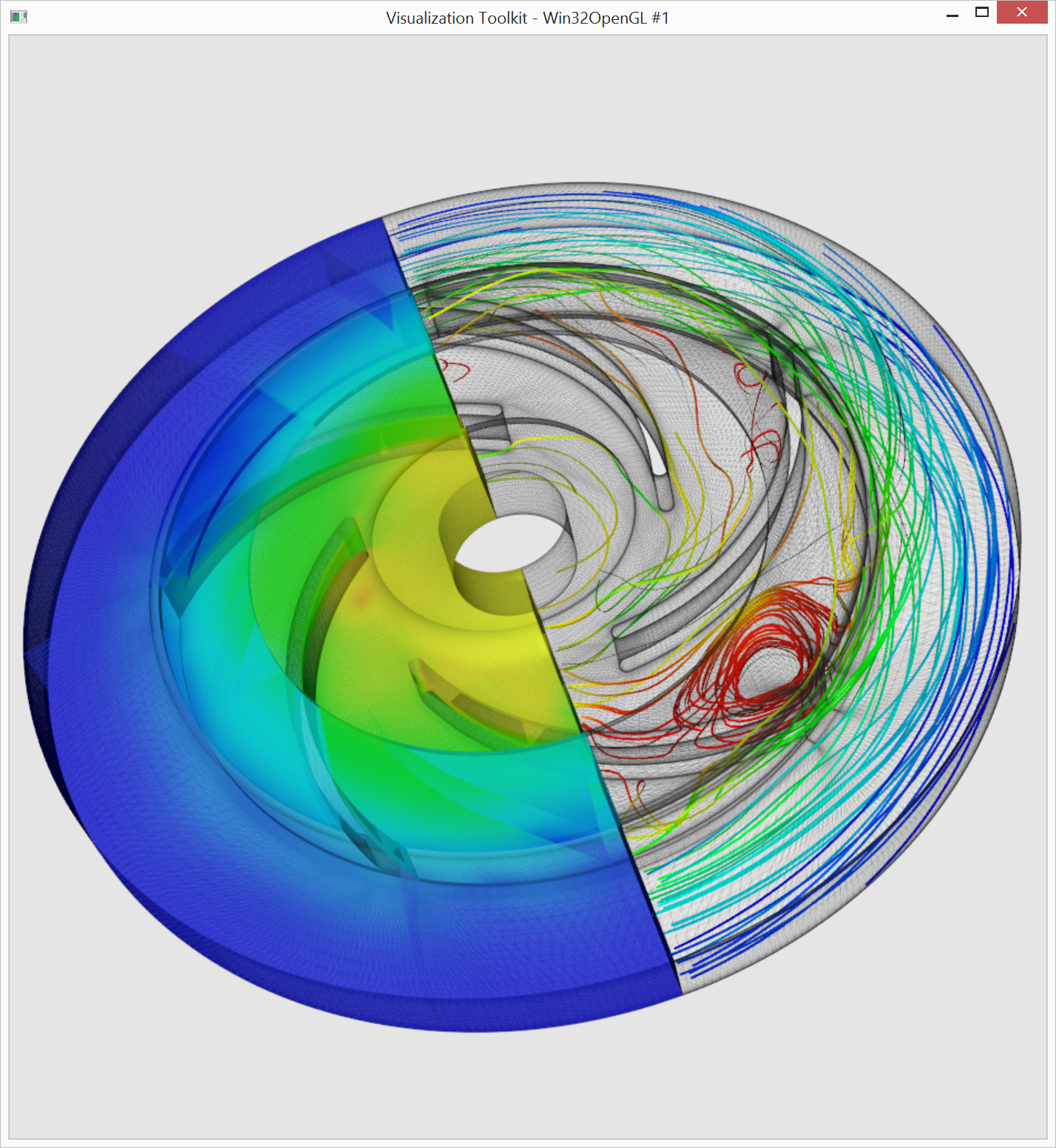
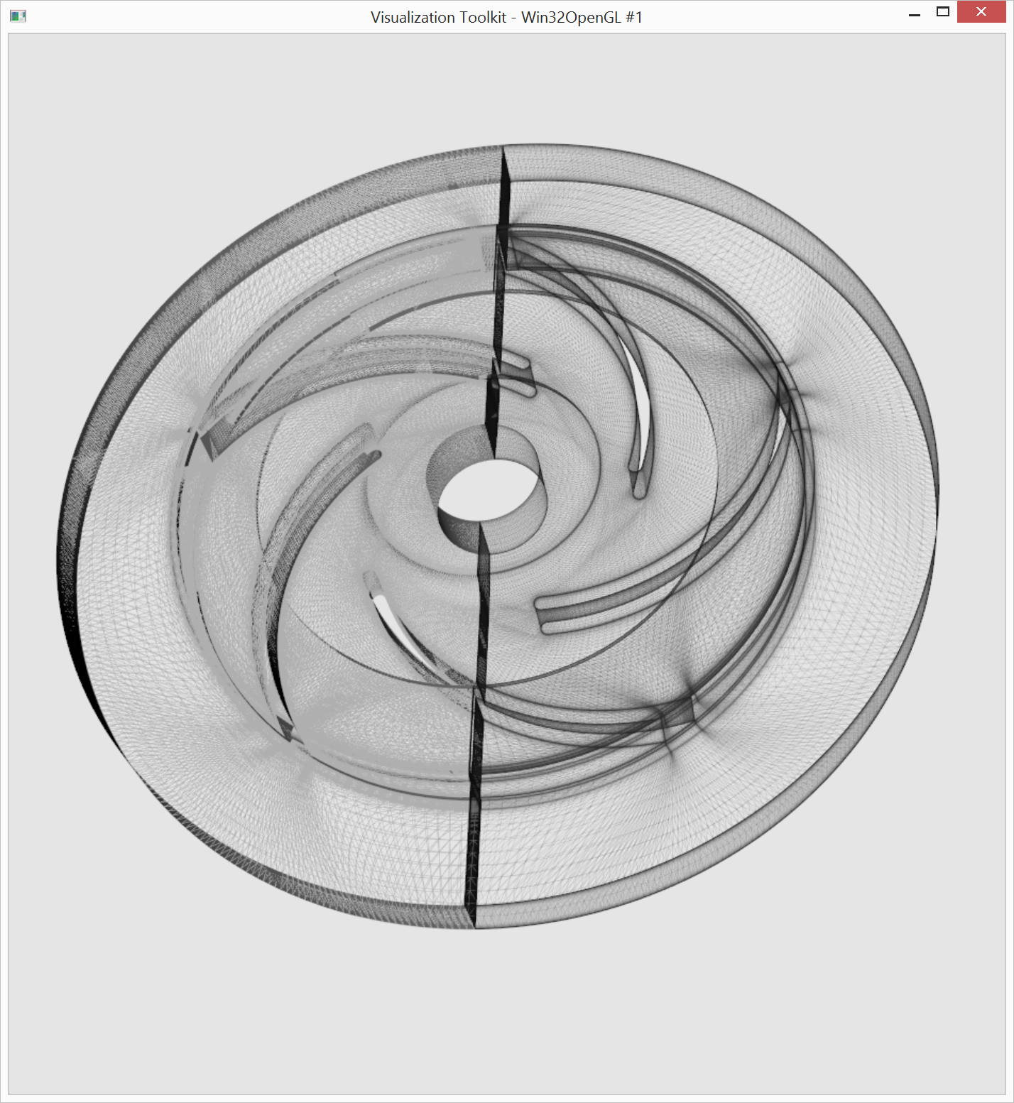
What we will achieve using VTK is the visualization shown in the image below. As a 3D context the outline of the dataset is shown using a partially transparent wireframe rendering. The left part of the dataset is then used to display the pressure using simple color coding of the surfaces. (We’ll skip the more complex volume rendering for this example). In order to visualize the velocity field, the right part of the dataset is filled with streamlines, which are color-coded by the magnitude of their velocity. This visualization choice is technically not ideal, but I wanted to keep the VTK code as simple as possible.
In addition, there is a reason for this example to be part of a visualization challenge, i.e., lots of turbulence in the flow.

Final Visualization of Fluid Flow in An Impeller Pump

Step by Step

I will discuss the VTK code step by step, showing how the rendering output would look at each stage. The full source code can be downloaded at the end of the article.

Let’s starts by including everything we need from VTK and open the main function.

#include <vtkActor.h>
#include <vtkArrayCalculator.h>
#include <vtkCamera.h>
#include <vtkClipDataSet.h>
#include <vtkCutter.h>
#include <vtkDataSetMapper.h>
#include <vtkInteractorStyleTrackballCamera.h>
#include <vtkLookupTable.h>
#include <vtkNew.h>
#include <vtkPlane.h>
#include <vtkPointData.h>
#include <vtkPointSource.h>
#include <vtkPolyDataMapper.h>
#include <vtkProperty.h>
#include <vtkRenderer.h>
#include <vtkRenderWindow.h>
#include <vtkRenderWindowInteractor.h>
#include <vtkRibbonFilter.h>
#include <vtkStreamTracer.h>
#include <vtkSmartPointer.h>
#include <vtkUnstructuredGrid.h>
#include <vtkXMLUnstructuredGridReader.h>

int main(int argc, char** argv) {

Next, we setup the renderer and the render window in order to display our results. We set the background color and the render window size.

// Setup the renderer
vtkNew<vtkRenderer> renderer;
renderer->SetBackground(0.9, 0.9, 0.9);

// Setup the render window
vtkNew<vtkRenderWindow> renWin;
renWin->AddRenderer(renderer.Get());
renWin->SetSize(500, 500);

With this code we could already display a static render window. Instead, we opt to add a vtkRenderWindowInteractor in order to interactively rotate, zoom and pan the scene.

// Setup the render window interactor
vtkNew<vtkRenderWindowInteractor> interact;
vtkNew<vtkInteractorStyleTrackballCamera> style;
interact->SetRenderWindow(renWin.Get());
interact->SetInteractorStyle(style.Get());

Now we have a running example showing a gray, empty render window.

Next, we load the dataset using one of the many readers that come with VTK.

// Read the file
vtkSmartPointer<vtkXMLUnstructuredGridReader> pumpReader = vtkSmartPointer<vtkXMLUnstructuredGridReader>::New();
pumpReader->SetFileName("rotor.vtu");

Short excursion into VTK memory management: VTK uses a convenient automatic memory management concept revolving around reference counting. Different from most other implementations however, the reference count is kept within the VTK objects themselves, instead of the smart pointer class. This has the advantage that the reference count can be increased, even if the VTK object is passed around as a raw pointer. There are two major ways to create managed VTK objects. vtkNew<T> and vtkSmartPointer<T>::New(), with the main difference being that a vtkSmartPointer<T> is implicit cast-able to the raw pointer T*, and can be returned from a function. For instances of vtkNew<T> we’ll have to call .Get() to obtain a raw pointer and we can only return it by wrapping it into a vtkSmartPointer. Within our example, we never return from functions and all objects live the whole time, therefore we’ll use the short vtkNew, with only the above exception for demonstration purposes.

At this point, nothing has been read from the file yet. We or a filter further down the chain would have to call Update() for the file reading to actually happen. It is usually the best approach to let the VTK classes handle the updates themselves. However, sometimes we want to access the result of a filter directly, for example to get the range of pressures in this dataset. Then we need to call Update() manually. (We don’t lose performance by calling Update() multiple times, as the results are cached.)

// Get the pressure range
pumpReader->Update();
double pressureRange[2];
pumpReader->GetOutput()->GetPointData()->GetArray("Pressure")->GetRange(pressureRange);

Next, we need to extract the left half of the dataset, using vtkClipDataSet. To achieve this we first define a vtkPlane that defines the split. Then, we’ll see for the first time how the VTK pipeline is connected together: successor->SetInputConnection(predecessor->GetOutputPort()). Whenever we request an update from clipperLeft this connection will now ensure that all preceding filters are also up to date.

// Clip the left part from the input
vtkNew<vtkPlane> planeLeft;
planeLeft->SetOrigin(0.0, 0.0, 0.0);
planeLeft->SetNormal(-1.0, 0.0, 0.0);

vtkNew<vtkClipDataSet> clipperLeft;
clipperLeft->SetInputConnection(pumpReader->GetOutputPort());
clipperLeft->SetClipFunction(planeLeft.Get());

Finally, we create our first actors and mappers to display the wireframe rendering of the left half. Notice, that the mapper is connected to its filter in exactly the same way as the filters to each other. Most of the time, the renderer itself is triggering the updates of all actors, mappers and the underlying filter chains!

The only line that is not self-explanatory is probably leftWireMapper->ScalarVisibilityOff(); –– it prohibits the coloring of the wireframe by pressure values, which are set as the currently active array.

// Create the wireframe representation for the left part
vtkNew<vtkDataSetMapper> leftWireMapper;
leftWireMapper->SetInputConnection(clipperLeft->GetOutputPort());
leftWireMapper->ScalarVisibilityOff();

vtkNew<vtkActor> leftWireActor;
leftWireActor->SetMapper(leftWireMapper.Get());
leftWireActor->GetProperty()->SetRepresentationToWireframe();
leftWireActor->GetProperty()->SetColor(0.8, 0.8, 0.8);
leftWireActor->GetProperty()->SetLineWidth(0.5);
leftWireActor->GetProperty()->SetOpacity(0.8);

renderer->AddActor(leftWireActor.Get());

At this point, the render window is finally showing something, i.e., the wireframe for the left part.

Wireframe of Left Part of Pump Data

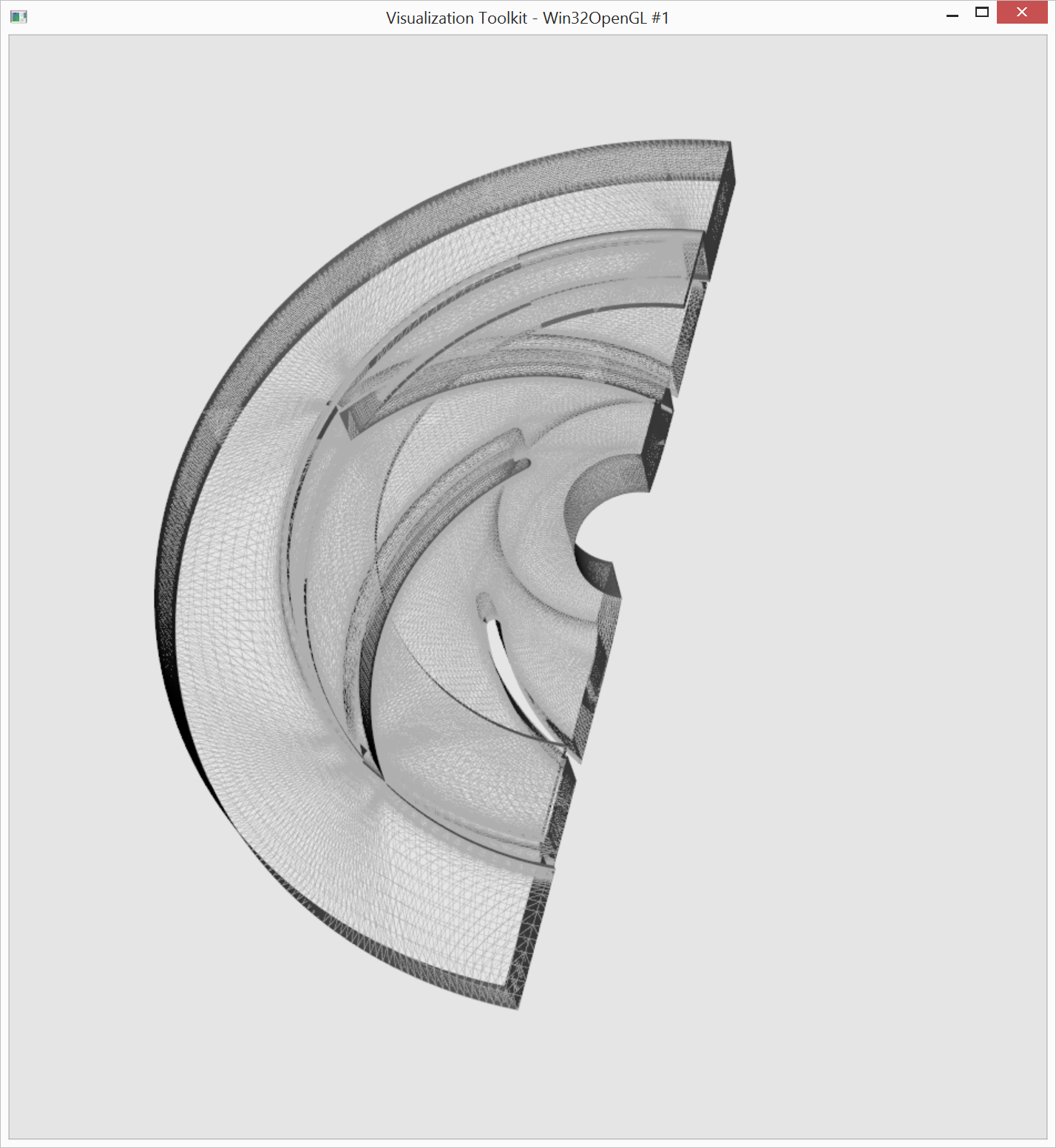
The wireframe rendering for the right part is created in a similar way, by switching the plane normal of a (newly created) vtkClipDataSet to the opposite direction and slightly changing the color and opacity of the (newly created) mapper and actor.
Notice, that here our VTK pipeline splits into two directions (right and left) from the same input dataset.

// Clip the right part from the input
vtkNew<vtkPlane> planeRight;
planeRight->SetOrigin(0.0, 0.0, 0.0);
planeRight->SetNormal(1.0, 0.0, 0.0);
vtkNew<vtkClipDataSet> clipperRight;
clipperRight->SetInputConnection(pumpReader->GetOutputPort());
clipperRight->SetClipFunction(planeRight.Get());

// Create the wireframe representation for the right part
vtkNew<vtkDataSetMapper> rightWireMapper;
rightWireMapper->SetInputConnection(clipperRight->GetOutputPort());
rightWireMapper->ScalarVisibilityOff();
vtkNew<vtkActor> rightWireActor;
rightWireActor->SetMapper(rightWireMapper.Get());
rightWireActor->GetProperty()->SetRepresentationToWireframe();
rightWireActor->GetProperty()->SetColor(0.2, 0.2, 0.2);
rightWireActor->GetProperty()->SetLineWidth(0.5);
rightWireActor->GetProperty()->SetOpacity(0.1);
renderer->AddActor(rightWireActor.Get());

The output window now shows both wireframe parts, as expected.

Wireframe of Left and Right Sides of Pump

Now we are ready to visualize some useful data! For adding the pressure visualization to the left part, we don’t need to do much. We create a new mapper and connect it to clipperLeft as well, but this time we color by the pressure array. It is also here, that we finally utilize the pressureRange we have derived above.

// Create the pressure representation for the left part
vtkNew<vtkDataSetMapper> pressureColorMapper;
pressureColorMapper->SetInputConnection(clipperLeft->GetOutputPort());
pressureColorMapper->SelectColorArray("Pressure");
pressureColorMapper->SetScalarRange(pressureRange);

vtkNew<vtkActor> pressureColorActor;
pressureColorActor->SetMapper(pressureColorMapper.Get());
pressureColorActor->GetProperty()->SetOpacity(0.5);

renderer->AddActor(pressureColorActor.Get());

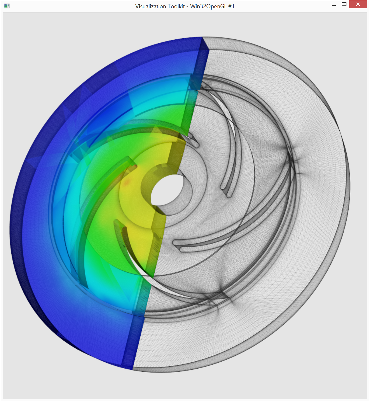
The output now looks like the image shown below. The pressure at the middle is very low, sucking material into the pump. Then, this material is transported to the outside, rapidly gaining pressure. (Of course there should be a color map legend with the actual values, but I left it out to keep the example shorter.)

Color Mapping Of Pressure in Pump

Now the trickier part starts. We want to draw velocity streamlines in the right part. Streamlines are generated by integration within a vector field from source points. The vector field is already part of the dataset in the form of the “Velocities” vector-array. So we only need to generate the source points. vtkPointSource generates a sphere of random points. We’ll generate 1500 source points, because most of them won’t lie within the dataset anyways and will be ignored by the stream tracer.

// Create the source points for the streamlines
vtkNew<vtkPointSource> pointSource;
pointSource->SetCenter(0.0, 0.0, 0.015);
pointSource->SetRadius(0.2);
pointSource->SetDistributionToUniform();
pointSource->SetNumberOfPoints(1500);

Next we create the streamtracer and set its input connections. “Wait, multiple connections?”, you might say. Yes – this is the first VTK filter with multiple inputs we encounter. The normal input connection is used for the vector field, and the source connection is used for the seed points. Since “Velocities” is the “active” vector array in clipperRight, we don’t need to specify it here explicitly. Finally we specify that the integration should be performed to both directions from the seed points, and set the integration method to Runge-Kutta-4.5.

vtkNew<vtkStreamTracer> tracer;
tracer->SetInputConnection(clipperRight->GetOutputPort());
tracer->SetSourceConnection(pointSource->GetOutputPort());
tracer->SetIntegrationDirectionToBoth();
tracer->SetIntegratorTypeToRungeKutta45();

Our next problem is coloring the streamlines by velocity magnitude. Since there is no array for the magnitudes of the vectors, we will simply compute the magnitudes into a new scalar array. As you have guessed, there is a VTK filter for this task as well: vtkArrayCalculator. It takes a dataset and outputs it unchanged, but adds exactly one array that is computed from one or more of the existing ones. We configure this array calculator to take the magnitude of the “Velocity” vector and output it as “MagVelocity”. Finally, we call Update() manually again, in order to derive the range of the new array.

// Compute the velocity magnitudes and create the ribbons
vtkNew<vtkArrayCalculator> magCalc;
magCalc->SetInputConnection(tracer->GetOutputPort());
magCalc->AddVectorArrayName("Velocity");
magCalc->SetResultArrayName("MagVelocity");
magCalc->SetFunction("mag(Velocity)");
magCalc->Update();

double magVelocityRange[2];
magCalc->GetOutput()->GetPointData()->GetArray("MagVelocity")->GetRange(magVelocityRange);

vtkStreamTracer directly outputs polylines and vtkArrayCalculator passes them on unchanged. Therefore we could just display the output of magCalc directly using a new mapper and actor.

Instead, we opt to make the output a little nicer, by displaying ribbons instead. vtkRibbonFilter generates 2D cells to display ribbons for all polylines of its input.

// Create and render the ribbons
vtkNew<vtkRibbonFilter> ribbonFilter;
ribbonFilter->SetInputConnection(magCalc->GetOutputPort());
ribbonFilter->SetWidth(0.0005);

vtkNew<vtkPolyDataMapper> streamlineMapper;
streamlineMapper->SetInputConnection(ribbonFilter->GetOutputPort());
streamlineMapper->SelectColorArray("MagVelocity");
streamlineMapper->SetScalarRange(magVelocityRange);

vtkNew<vtkActor> streamlineActor;
streamlineActor->SetMapper(streamlineMapper.Get());
renderer->AddActor(streamlineActor.Get());

What is now still missing, and is actually needed to produce the intermediate renderings as well, are the last five lines to actually render the scene and initialize the interactor.

// Render and show interactive window
renWin->Render();
interact->Initialize();
interact->Start();
return 0;
}

Finally, we arrive at the finished visualization, which I will present once again here:

Final Visualization of Fluid Flow in An Impeller Pump

The full source code for the above visualization can be found here.

The Good, the Bad, and the Ugly

I will close this article with a list of my personal pros and cons of the VTK framework.

• Pro: Active development: VTK is under active development from several contributors, mainly from within the research community. This means that some cutting-edge algorithms are available, many 3D-formats can be imported and exported, bugs are actively fixed, and problems usually have a ready-made solution in the discussion boards.

• Con: Reliability: Coupling many algorithms from different contributors with the open pipeline design of VTK however, can lead to problems with unusual filter combinations. I have had to go into the VTK source code a few times in order to figure out why my complex filter chain is not producing the desired results. I would strongly recommend setting up VTK in a way that permits debugging.

• Pro: Software Architecture: The pipeline design and general architecture of VTK seems well thought out and is a pleasure to work with. A few code lines can produce amazing results. The built-in data structures are easy to understand and use.

• Con: Micro Architecture: Some micro-architectural design decisions escape my understanding. Const-Correctness is almost non-existent, arrays are passed around as inputs and outputs with no clear distinction. I alleviated this for my own algorithms by giving up some performance and using my own wrapper for vtkMath which utilizes custom 3D types like typedef std::array<double, 3> Pnt3d;.

• Pro: Micro Documentation: The Doxygen documentation of all classes and filters is extensive and usable, the examples and test cases on the wiki are also a great help to understand how filters are used.

• Con: Macro Documentation: There are several good tutorials for and introductions to VTK on the web. However as far as I know, there is no big reference documentation that explains how specific things are done. If you want to do something new, expect to search for how to do it for some time. In addition it is hard to find the specific filter for a task. Once you’ve found it however, the Doxygen documentation will usually suffice. A good way to explore the VTK framework is to download and experiment with Paraview.

• Pro: Implicit Parallelization Support: If your sources can be split into several parts that can be processed independently, parallelization is as simple as creating a separate filter chain within each thread that processes a single part. Most large visualization problems usually fall into this category.

• Con: No Explicit Parallelization Support: If you are not blessed with large, dividable problems, but you want to utilize multiple cores, you are on your own. You’ll have to figure out which classes are thread-safe, or even re-entrant by trial-and-error or by reading the source. I once tracked down a parallelization problem to a VTK filter that used a static global variable in order to call some C library.

• Pro: Build system CMake: The multi-platform meta-build-system CMake is also developed by Kitware (the makers of VTK) and used in many projects outside of Kitware. It integrates very nicely with VTK and makes setting up a build system for multiple platforms much less painful.
• Pro: Platform Independence, License, and Longevity: VTK is platform independent out of the box, and is licensed under a very permissive BSD-style license. In addition, professional support is available for those important projects that require it. Kitware is backed by many research entities and other companies and will be around for some time.

Last Word

Overall, VTK is the best tool for the kinds of problems I love. If you ever come across a project that requires visualization, mesh processing, image processing or similar tasks, try firing up Paraview with an input example and evaluate if VTK could be the tool for you.